propagation of errors, calibration, random errors

This website contains other cold fusion items.
Click to see the list of links br>

An illustration of calibration

Ludwik Kowalski (August 5, 2007)
Montclair State University, Montclair, N.J. 07055

It often happens that a physical quantity in which we are interested depends on several quantities, x, y, z, which we measure. We say that the quantity is a function of (x,y,z). Sometimes this function is known. For example, the density of a cylinder can be calculated from D = mass/volume. In that case the formula is

D =4*m/(3.145*d^2*h)

where m is the mass, d is the diameter and h is the height. The m, d and h are measured and D is calculated. The well known rules of propagation of errors (1) can then be used to calculate the uncertainty (random error) associated with the calculated quantity. If the errors in m, d and h are, 2%, 3% and 1%, for example, then the uncertainty associated with the calculated density is close to 4.8%. A situation is not as simple when a formula to calculate the value of the quantity of interest is not known. In such case a researcher must depend on calibration. What follows describes an example of a calibration for a simple case in which the quantity of interest is a function of only one variable. I will ignore procedures used to deal with propagation of errors (via calibration) when the quantity depends on more than one variable.

Suppose we are studying an alloy of copper and zinc. We know that the resistivity, r, depends on the percentage of zinc, p. We want to be able to calculate p from r, after r is measured, But the formula for p(r) relation is not known. We also want to be able to calculate the uncertainty associated with the calculated p. To accomplish this we prepare six cylindrical samples of the alloys of known p. The values of p, for these standards of reference, are 5, 10, 15, 20, 25 and 30 percent. We measure r for each of these these samples and obtain the following set of data:

  p(% of Zn)    5.0     10      15     20      25     30  
  r(nΩ*m)      31.2    32.7   38.1    53.1   58.4   52.4

For pure copper, at room temperature, r would probably be close to 1.68*10^-8Ω*m (16.8 nΩ*m) as reported in most textbooks. The linear regression line, for these six calibration points, happens to be:

p = 0.721*r - 14.5

as illustrated in Figure 1a. That is the end of calibration; the linear relation above becomes our formula to calculate p after r is measured. Details about the method used to measue r are not important in this context. The only important thing is the limited precision of measurements.

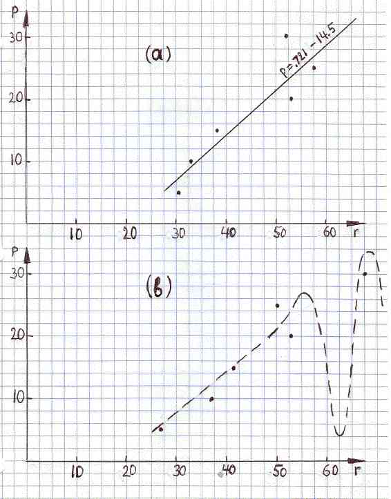
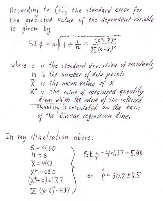
FIGURE 1ab
(a) Calibration scatter plot, p versus r, and the linear regression line.
(b) Another possible scatter plot, after remeasuring r for the same set of six standard alloys. The dashed line shows a possible nonlinear relation between p and r.
- - - - - - - - - - - - - - - -
For example, suppose a sample of unknown composition is given to us. We measure its resistivity and the result is 62.0 nΩ*m. What is the percentage of zinc in that sample? Using the above correlation line we find that p is 30.2 percent. And what uncertainty should be assigned to this results? Looking at the Figure 1a, we see that some data points are above the regression line while others are below it. This is due to random errors associated with measurements of r. The six numbers below are vertical distances between data points and the calibration line (see Figure 1a).

  dp (% Zn):   -3.04    +0.881   +1.98   -3.83   -2.66   +6.67

Such differences are often called residuals. Note that the mean value of residuals is essentially zero, as is should be according to the definition of the correlation line. Positive numbers refer to data points above the line while negative numbers refer to points below the line. It should be intuitively clear that the uncertainty in p would be larger if random fluctuations of data points, with respect to the correlation line, were larger. Smaller fluctuations, on the other hand, would indicate that the random error in p is smaller. The standard deviation, s, of the above six residuals is 4.00. The uncertainty in p, proportional to s, is thus 5.5, as illustrated in Figure 2.

The above method of inference, however, is not universal. Suppose the true relation between p and r is as shown by the dashed line in Figure 1b. That hypothetical relation has a deep minimum near r=0.62. Not being aware of the minimum we would say that p is 30, plus or minus 4 percent. But real p would be much smaller. The method described above should be used only when one is reasonably sure, on the basis of additional information, that the true relation between the variables is not very different from its linear approximation. ( Any non linear function can be approximated by a line segment for a sufficiently narrow range of independent variable.)

The six data points in Figure 1b is the result of another calibration, based on the same six standards as in Figure 1a. The new numerical data are show below.

  p(% of Zn)       5.0     10     15     20     25     30  

  r(nΩ*m)         26.1    35.7   41.1  52.8   50.2   67.6

This time the calibration line turns out to be

p = 0.622*r - 10.9

It coincides with the dashed line in Figure 2b only when r<4.5 . Why is this line slightly different from the one we obtained before? This is due to the limited precision of measuring r. Note that we are assuming that errors in p, for standards of reference, were negligible. According to the new calibration line, the value of p, assigned to 62 nW*m, should be 27.7 percent (plus or minus of approximately 1,5%Zn), rather than 32 percent (plus or minus approximately 4%Zn), as before. Ambiguities of that kind are unavoidable because results of measurements fluctuate around true values. Two kinds of related ambiguities can be recognized in our situation; one about the exact location of the calibration line, and another about values of p based on single measurements of r.

Figure 2
The term (x* - x_bar), under the square root, is the horizontal component of the distance of a particular value of x* from the central region. The uncertainty assigned to the inferred value is at a minimum when the measured value x* is closer to the center. Note that x*=62 is located near the right-hand margin of the scatter plot. For an x* close to 44.3, the third term under the square root would become negligible. Furthermore, the second term becomes negligible when n>20. Thus, for a large number of calibration points, the uncertainty in the inferred value approaches the standard deviation of residuals when x* approaches the mean x. This is intuitively acceptable; try to totate the regression line about the centroid of data points, (x_bar,y_bar). The range of calibration data points should not be limited to the range of expected values of x*, the wider the calibration range the smaller the uncertainty assigned to p, for any given n.

P.S.
This note was inspired by correspondence with Scott Little, a calorimetrist who uses linear regression calibrations. The correspondence, in turn, was triggered by Scott's paper (2), and by comments made by several CMNS researchers (3). Scott also critically examined my original draft and helped to improve it. But his method of calculating uncertainties is based on commercial software.

References:
1) David Moore, “The Basic Principles of Statistics,” 2nd edition, Freeman, 2000, page 544.
Keep in mind that I am not a statistician. I will be happy to add a clearly written appendix with results based on alternative formulas, and on commonly available software.

2) Scott R. Little “Null Tests of Breakthrough Energy Claims,” Presented at “42nd AIAA/ASME/SAE/ASEE Joint Propulsion Conference & Exhibit , 9 - 12 July 2006, Sacramento, California.”
Link to the paper http://www.earthtech.org/publications/index.html (click on item #6).

3) Comments on Scott's paper, made by several CMNS researchers, including Scott himself, were published by S. Krivit, in the 23th issue of New Enenrgy Times, July 10, 2007
Link to Krivit's publication: http://newenergytimes.com/news/2007/NET23.html